
Analysis of Candidate Landing Sites for Future Mars Rover Missions
A project as involved as this one requires a lot of data processing and pre-processing. The purpose of this page is to document the various analysis steps that were necessary to be able to conduct the suitability analysis, and subsequently interpret and display the results. The workflow can roughly be broken down into three stages: i) pre-processing of raw data to generate raster datasets that can be used in the suitability analysis; ii) reclassification of the various rasters used in the suitability analysis and addition of them to generate the initial suitability raster; and iii) interpretation and display of the results.
1. Pre-Processing of Raw Data
For this project I obtained a total of 13 individual raw datasets, in a variety of formats. These datasets are tabulated below, with weblinks and abbreviations provided in the footnote*.
| Dataset | Source | Date of Retrieval |
|---|---|---|
| MOLA Elevation Raster | NASA Planetary Data System (PDS) | 28/04/2020 |
| TES Albedo Raster | NASA PDS | 28/04/2020 |
| TES Thermal Inertia Raster | NASA PDS | 28/04/2020 |
| TES Carbonate Raster | NASA PDS | 28/04/2020 |
| TES Hematite Raster | NASA PDS | 28/04/2020 |
| TES Sulfate Raster | NASA PDS | 28/04/2020 |
| OMEGA Hydrous Mineral Database | ESA Planetary Science Archive | 26/05/2020 |
| Open-Basin Crater Lake Database | Integrated Database of Planetary Features (IDPF) | 14/05/2020 |
| Closed-Basin Crater Lake Database | IDPF | 14/05/2020 |
| Valley Network Database | IDPF | 14/05/2020 |
| Delta Database | IDPF | 14/05/2020 |
| Polygonal Ridge Database | IDPF | 14/05/2020 |
| Global Geologic Map | USGS Publication SIM 3292 | 17/01/2020 |
These datasets were obtained in a variety of formats, including existing raster data, shapefile polygon and polyline datasets, and simple .csv file xy coordinates. To conduct the suitability analysis I required a suite of rasters of the same cell size with all the cells correctly aligned. The MOLA elevation dataset (DEM) is the highest resolution (i.e., smallest cell size; ~ 463 m/pixel) global Martian dataset available. Thus, I chose to use this as my common starting point and aligned everything else to it. All existing raster data were resampled to the cell size of the MOLA DEM and snapped to it. A slope raster was derived from the elevation DEM also. Additionally, a constant raster was created with the extent and cell size of the DEM, and subsequently extracted multiple times to create the following latitude band rasters: > 45°N and S, 30°N to 45°N, 30°N to 15°S, 15°S to 30°S, 30°S to 45°S.
The existing raster datasets with global coverage (TES albedo, TES thermal inertia, and the three TES mineral abundance maps – carbonate, hematite, and sulfate) were all resampled to the cell size of the elevation DEM and snapped to it.
The valley network dataset was a shapefile of polylines representing features identified as fluvial (i.e., river-carved) channels. A distance raster (to a maximum of 25 km) was created for this dataset and resampled to the cell size of the elevation DEM and snapped to it.
The datasets representing features interpreted as delta deposits, as well as the locations at which hydrous minerals (such as clays) had been observed, were point feature class datasets. Distance rasters (again to 25 km) were created for both, and resampled to the cell size of the elevation DEM and snapped to it.
The polygonal ridge dataset contained polygons of regions in which polygonal ridge landforms had been identified. A subset of these, those that are believed to have an origin involving subsurface water flow, were selected and used to create another distance raster. Once again the distance raster was capped at 25 km and resampled to the cell size of the elevation DEM and snapped to it.
The final dataset that needed processing was the point feature class dataset for the open-basin and closed-basin crater lakes. The raw dataset identified, with simple points, craters which are thought to have contained lakes at some point in the past. To get this dataset into a suitable raster format a point feature class global crater database was restricted to those craters larger than 25 km in diameter but smaller than 500 km. These craters were then buffered by their radius to create spherical polygons approximately the same size and shape as the craters. The closed-basin point feature class was spatially joined to this crater dataset and craters that were not null (i.e., those craters containing a closed-basin lake point) were selected and exported as a new feature class. This subset of craters was used to create a distance raster to a maximum of 25 km, and this was resampled to the cell size of the elevation DEM and snapped to it. The same process was repeated with the open-basin lake dataset. This pre-processing step resulted in 18 separate raster datasets, each one with the same cell size as the elevation DEM and all snapped to that raster for alignment.
2. Conducting The Suitability Analysis
Once all the raw data that I had accumulated had been converted into a suitable format, I had to reclassify that data and add all the resulting rasters together. This is the stage where you, as the analyst, can decide which criteria should have more or less weight in the final analysis. The ModelBuilder model used for this process is illustrated below.
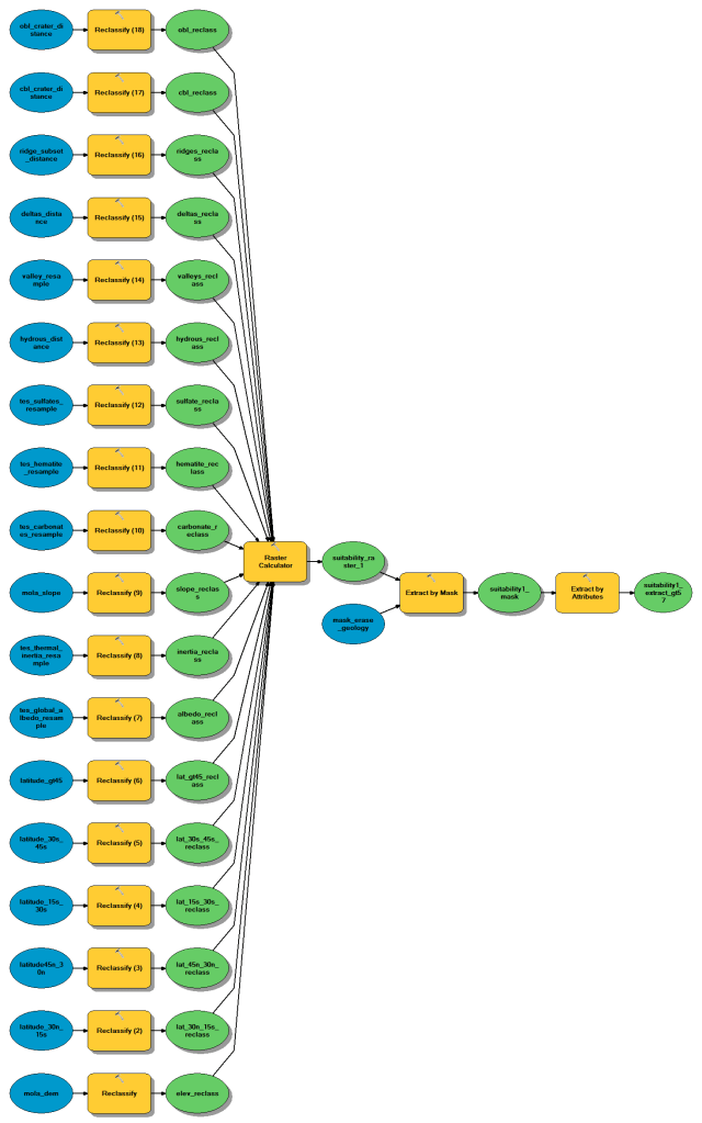
The reclassification values used in the model above are summarized in the table below. For simplicity, during the first run I kept the weighting of most criteria equal – with a highest score of 10, decreasing to 6, then 4, and finally 0. For a few features I reduced this scale by a factor of 2, such that the maximum score was 5 rather than 10. An advantage of constructing a ModelBuilder model to accomplish this task is that it is relatively straightforward to change these values and re-run the analysis.
| Criterion | Initial Value(s) | Reclassified Value |
|---|---|---|
| Elevation | ≥ +2000 m | 0 |
| +2000 to 0 m | 4 | |
| 0 to -2000 m | 6 | |
| ≤ -2000 m | 10 | |
| Latitude | ≥ 45°N or S | 0 |
| 30°S to 45°S | 4 | |
| 45°N to 30°N | 6 | |
| 15°S to 30°S | 6 | |
| 30°N to 15°S | 10 | |
| Slope | ≥ 30° | 0 |
| 30° to 15° | 4 | |
| 15° to 5° | 6 | |
| < 5° | 10 | |
| Albedo | ≥ 0.25 | 0 |
| < 0.25 | 10 | |
| Thermal Inertia | < 100 | 0 |
| units of J m-2 S-0.5 K-1 | 100 to 150 | 6 |
| ≥ 150 | 10 | |
| Carbonate Abundance | < 0.1 | 0 |
| > 0.1 | 10 | |
| Hematite Abundance | < 0.1 | 0 |
| > 0.1 | 10 |
| Criterion | Initial Value(s) | Reclassified Value |
|---|---|---|
| Sulfate Abundance | < 0.1 | 0 |
| > 0.1 | 10 | |
| Hydrous Minerals | ≥ 25 km | 0 |
| 25 to 15 km | 4 | |
| 15 to 5 km | 6 | |
| < 5 km | 10 | |
| Valley Networks | ≥ 25 km | 0 |
| 25 to 15 km | 4 | |
| 15 to 5 km | 6 | |
| < 5 km | 10 | |
| Deltas | ≥ 25 km | 0 |
| 25 to 15 km | 4 | |
| 15 to 5 km | 6 | |
| < 5 km | 10 | |
| Polygonal Ridges | ≥ 25 km | 0 |
| 25 to 15 km | 2 | |
| 15 to 5 km | 3 | |
| < 5 km | 5 | |
| Closed-Basin Lakes | > 1 km | 0 |
| < 1 km | 5 | |
| Open-Basin Lakes | > 1 km | 0 |
| < 1 km | 5 |
3. Interpretation
Once these rasters had been summed I was left with a single global raster, with 463 m pixels, with each pixel or cell having a score between 0 and a theoretical maximum of 125. However, there are regions of the planet that are not suitable for landing or operating a rover in. Some of these, representing high latitudes or elevations, received scores of zero during reclassification. Others, such as constraints on the geology provided by the geologic map, were not included in the suitability raster. The first step in the interpretation of the data was the construction of a ‘mask’, which would extract from the initial suitability raster only those cells in certain regions of the planet.
The criteria for inclusion in the final analysis are: i) latitude less than 45°N or S; ii) elevation less than +2000 m; iii) albedo less than 0.25; and iv) thermal inertia greater than 100 J m-2 s-0.5 K-1. To prepare the mask polygon, an initial polygon representing the 45°N to 45°S region was created. Next those portions of the elevation, albedo, and thermal inertia rasters not meeting the above criteria were selected with the set null tool and converted to polygons. These polygons were then sequentially erased from the initial latitude polygon.
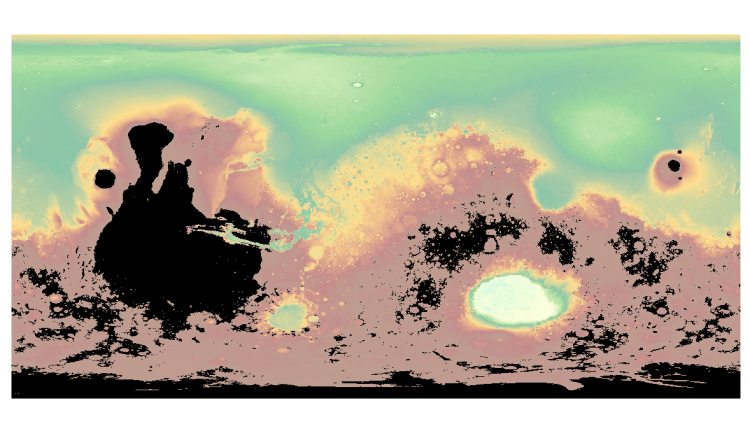
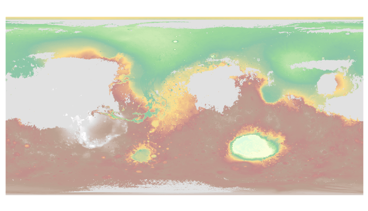
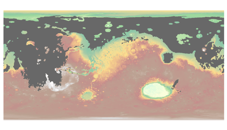
The final step in preparing the mask involved erasing a few additional regions that had been identified on the geologic map as being unsuitable. These regions (such as young volcanic provinces and the relatively young northern lowlands) had already largely been eliminated by the other criteria. The geologic map polygons representing these unwanted geologic units were selected by attribute and dissolved into a single polygon, which was subsequently erased from the mask polygon. This mask polygon was then used to extract only the suitable cells from the suitability raster. The image below is a colour elevation model, with unsuitable areas masked out. Only cells in the remaining coloured region were included in the analysis of the results.
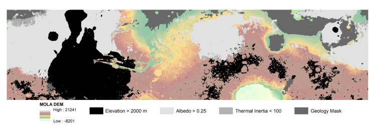
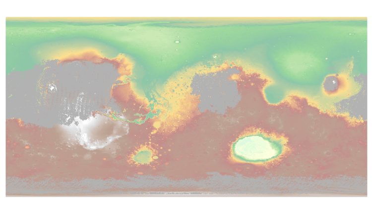
The individual extents of the elevation, albedo, thermal inertia, and geology masks are illustrated in the panels below.
The final step was to identify the highest scoring sites from the masked suitability raster that remained. The initial global raster contained more than 1 billion individual cells, of which ~ 245 million cells remained after applying the mask. The top 0.75% of these (~ 1.85 million cells) were extracted by value as the most suitable candidate landing sites.
The extracted subset of cells were converted to polygons, yielding over 14,000 individual polygons, and sorted into descending order by score. Regions of adjacent polygons were manually selected and named, beginning with the highest scoring polygons. By the time all regions with a maximum score of 66 or more had been grouped and named, a total of 8510 of the 14,047 polygons had been included and named (60.5%). These highest scoring regions were dissolved on the name field to yield polygons representing 88 separate regions. In the next section I will take a look at the characteristics of these regions and evaluate how well my analysis identified sites that have been considered by NASA and the wider planetary community as candidate sites for actual Mars missions.
